Scale Bars

This guide is structured like a tutorial, in order to showcase the various options and methods available; if you would like to follow along, a few additional packages and set-up steps are required:

Set-Up¶

# Packages used by this tutorial
import geopandas # manipulating geographic data
import numpy # creating arrays
import pygris # easily acquiring shapefiles from the US Census
import matplotlib.pyplot # visualization

# Downloading the state-level dataset from pygris
states = pygris.states(cb=True, year=2022, cache=False).to_crs(3857)

# This is just a function to create a new, blank map with matplotlib, with our default settings
def new_map(rows=1, cols=1, figsize=(5,5), dpi=150, ticks=False):
    # Creating the plot(s)
    fig, ax = matplotlib.pyplot.subplots(rows,cols, figsize=figsize, dpi=dpi)
    # Turning off the x and y axis ticks
    if ticks==False:
        if rows > 1 or cols > 1:
            for a in ax.flatten():
                a.set_xticks([])
                a.set_yticks([])
        else:
            ax.set_xticks([])
            ax.set_yticks([])
    # Returning the fig and ax
    return fig, ax

The above is only necessary for this specific tutorial; below, we import the main elements related to scale bars:

# Importing the main package
from matplotlib_map_utils import ScaleBar, scale_bar

Creating a Scale Bar¶

Don't Change Figure DPI After Creation

Your desired DPI must be set upon creation of the subplots/axes (ex., when calling matplotlib.pyplot.subplots(... dpi=##)), and not changed when saving the figure (e.x. when calling matplotlib.pyplot.savefig(... dpi=##)). This is because the scale bar is rasterized to match the current DPI of the figure upon creation - changing it later will mess up the scale and make the bar blurry (see this issue for more details).

Using the `scale_bar()` function¶

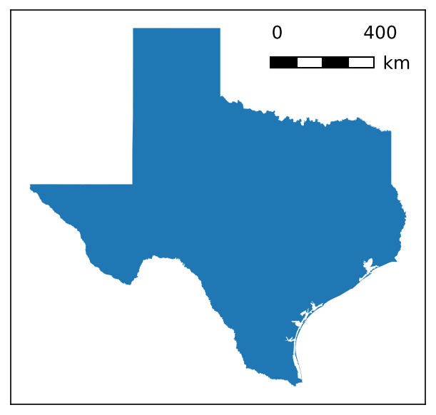
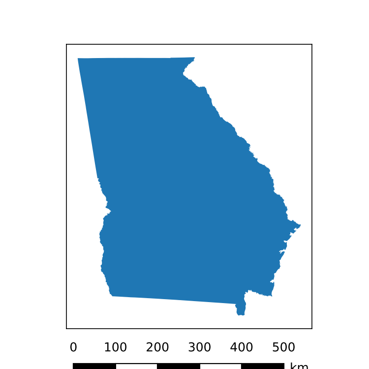
The quickest and easiest way to add a scale bar to a single plot is using the scale_bar() function. This will automatically create the artist and apply it to the supplied axis.

# Setting up a plot
fig, ax = new_map()

# Plotting a state (Georgia)
states.query("NAME=='Georgia'").plot(ax=ax)

# Adding a scale_bar to the upper-right corner of the axis - note that bar['projection'] MUST be set for this to work
scale_bar(ax=ax, location="upper right", style="boxes", bar={"projection":3857,"minor_type":"none"}, labels={"style":"first_last"})

a plot of Georgia with a scale bar added

Using the `ScaleBar` class¶

Alternatively, a ScaleBar class (based on matplotlib.artist.Artist) is also provided that allows the same bar to be rendered like so:

# Setting up a plot
fig, ax = new_map()

# Plotting a state (Georgia)
states.query("NAME=='Georgia'").plot(ax=ax)

# Creating a ScaleBar object that we want to place in the upper-right corner of the axis, 
# Note that here, we do not specify the axis
sb = ScaleBar(location="upper right", style="ticks", bar={"projection":3857,"minor_type":"none"}, labels={"style":"first_last"})

# The ScaleBar can then be added using add_artist(), which calls its built-in draw() function:
ax.add_artist(sb)

a plot of Georgia with a scale bar added

Re-using Objects¶

The benefit of the ScaleBar object is that it can be re-used across multiple plots without copy-pasting the function call. This is particularly beneficial for highly-customized bars: you can simply set it up once, and then add it to each axis you want.

The caveat to this is that instead of using ax.add_artist(ScaleBar), you have to use ax.add_artist(ScaleBar.copy()); as matplotlib does not let you add the same artist to multiple axes, you have to add a copy of the artist.

InvalidValid

Here, we try and re-use the sb artist we created above, which has already been applied to the plot of Georgia

# Setting up a plot
fig, ax = new_map()

# Plotting a new state (Texas)
states.query("NAME=='Texas'").plot(ax=ax)

# Trying to re-use the same artist - this will throw an error
ax.add_artist(sb)

Returns:

ValueError Can not reset the Axes. You are probably trying to reuse an artist in more than one Axes which is not supported

Now, we're starting from scratch:

# Setting up plots for both Georgia and Texas
ga_fig, ga_ax = new_map()
tx_fig, tx_ax = new_map()

# Plotting each state
states.query("NAME=='Georgia'").plot(ax=ga_ax)
states.query("NAME=='Texas'").plot(ax=tx_ax)

# Setting up the scale bar artist 
sb = ScaleBar(location="upper right", style="boxes", bar={"projection":3857,"minor_type":"none"}, labels={"style":"first_last"})

# Applying the artist to each plot
# Note we have to call .copy() EACH TIME
ga_ax.add_artist(sb.copy())
tx_ax.add_artist(sb.copy())

Returns:

a plot of Georgia with a scale bar added

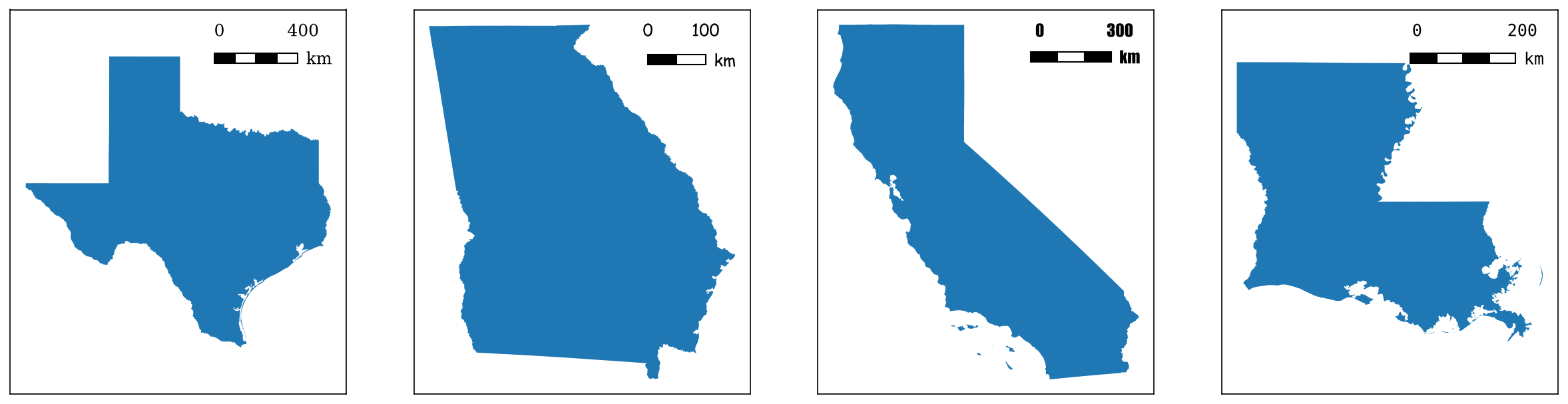
As you can see from the valid example, the bar updates its context across each plot it is applied to - the length and divisions updated to reflect the fact that Texas is a bigger state, but the formatting and appearance stayed the same.

Updating Objects¶

The customization options of the ScaleBar can be accessed using dot notation (like sb.base, sb.label, etc.). They can also be updated from this dot notation by passing a valid style dictionary (see next section for details).

Accessing ValuesUpdating Values

# Showing the labels style options
sb.labels

Returns:

{'style': 'first_last'}

# Updating the label style option for "loc"
sb.labels = {"loc":"above"}
sb.labels

Returns:

{'style': 'first_last', 'loc': 'above'}

This means you can update the properties of the created class while it is in use, in case you want small changes made in between iterations:

shapes = ["Texas","Georgia","California","Louisiana"]
# What we'll be updating
families = ["serif", "cursive", "fantasy", "monospace"]

# Creating the initial bar
sb = ScaleBar(location="upper right", style="boxes", bar={"projection":3857,"minor_type":"none"}, labels={"style":"first_last"})

# Creating four subplots
fig, axs = new_map(1,4, figsize=(20,5))
for ax,s,f in zip(axs.flatten(), shapes, families):
    states.query(f"NAME=='{s}'").plot(ax=ax)
    ax.set_aspect(1, adjustable="datalim")
    sb.text = {"fontfamily":f}
    ax.add_artist(sb.copy())

demonstrating changing the font family of the text attached to the scale bar

Though for this specific example, you could accomplish the same with the scale_bar() function just as (more?) easily

shapes = ["Texas","Georgia","California","Louisiana"]
families = ["serif", "cursive", "fantasy", "monospace"]

# Creating four subplots
fig, axs = new_map(1,4, figsize=(20,5))

for ax,s,f in zip(axs.flatten(), shapes, families):
    states.query(f"NAME=='{s}'").plot(ax=ax)
    ax.set_aspect(1, adjustable="datalim")
    scale_bar(ax=ax, location="upper right", style="boxes", bar={"projection":3857,"minor_type":"none"}, labels={"style":"first_last"}, text={"fontfamily":f})

demonstrating changing the font family of the text attached to the scale bar

Customizing the Scale Bar¶

Both the functional and object-oriented approach use the same primitive style dictionaries, so you can treat the following information as valid for both.

Specifying Length¶

There are three main ways of specifying the length of a scale bar, which utilizes the bar argument of the construction function or class method (see under Visible Components, below):

Physical / Plot LengthMaximum UnitsMajor Divison

length is used to set the total length of the bar, either in inches (for values >= 1) or as a fraction of the axis (for values < 1).

The default value of the scale bar utilizes this method, with a length value of 0.25 (meaning 25% of the axis).
It will automatically orient itself against the horizontal or vertical axis when calculating its fraction, based on the value supplied for rotation.
Values major_div and minor_div are ignored, while a value for max will override length.

Warning

Note that any values here will be rounded to a "nice" whole integer, so the length will always be approximate; ex., if two inches is 9,128 units, your scale bar will end up being 9,000 units, and therefore a little less than two inches.

max is used to define the total length of the bar, in the same units as your map, as determined by the value of projection and unit.

Ex: If you are using a projection in feet, and give a max of 1000, your scale bar will be representative of 1,000 feet.
Ex: If you are using a projection in feet, but provide a value of meter to unit, and give a max of 1000, your scale bar will be representative of 1,000 meters.
Will override any value provided for length, and give a warning that it is doing so!
Values can be optionally be provided for major_div and minor_div, to subdivide the bar into major or minor segments as you desire; if left blank, values for these will be calculated automatically (see preferred_divs in validation/scale_bar.py for the values used).

major_mult can be used alongside major_div to derive the total length: major_mult is the length of a single major division, in the same units as your map (as determined by the value of projection and unit), which is then multiplied out by major_div to arrive at the desired length of the bar.

Ex: If you set major_mult to 1,000, and major_div to 3, your bar will be 3,000 units long, divided into three 1,000 segments.
This is the only use case for major_mult - using it anywhere else will result in warnings and/or errors!
Specifying either max or length will override this method!
minor_div can still be optionally provided.

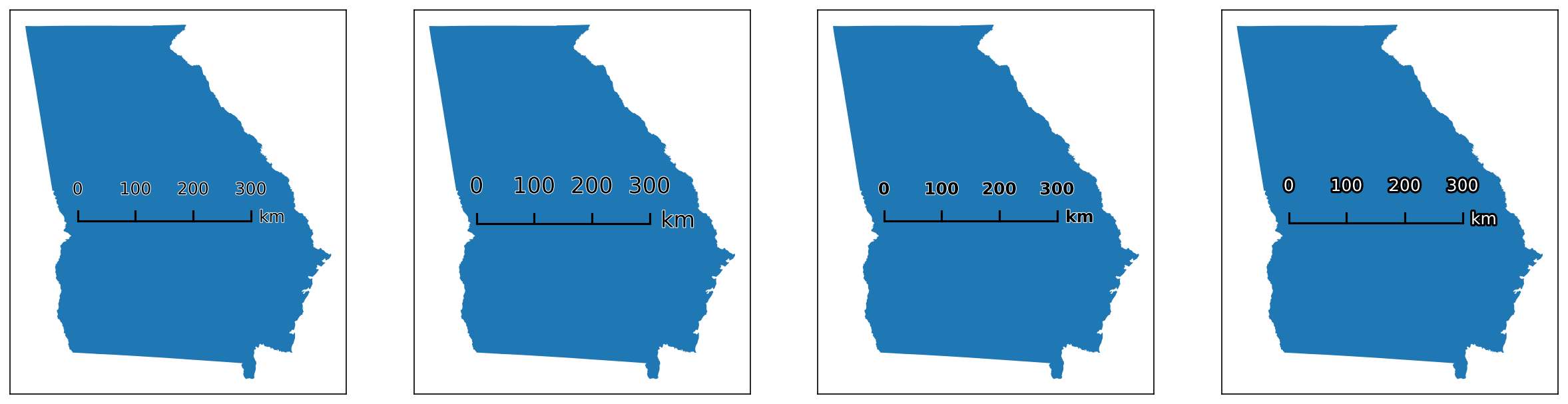
# Creating three identical bars using the four different methods
# Grid of location options
# Note that the "center" options will feel slightly off: this is because the the center of the scale bar is of the entire artist, text included, not just the bar itself
bar_lengths = [
    {"length":0.5}, # this bar will be ~50% of the axis
    {"length":2}, # this bar will be ~2.5 inches
    {"max":300, "major_div":3}, # this bar will be 300 km (because EPSG:3857 is in meters)
    {"major_mult":100, "major_div":3}, # this bar will be 300 km (100 * 3 = 300)
]

fig, axs = new_map(1,4, figsize=(20,5))

for ax,l in zip(axs.flatten(), bar_lengths):
    states.query(f"NAME=='Georgia'").plot(ax=ax)
    ax.set_aspect(1, adjustable="datalim")
    scale_bar(ax=ax, location="center", style="boxes", bar={"projection":3857,"minor_type":"none"} | l, labels={"style":"first_last"})

a repeated plot of Georgia with scale bars of similar lengths overlain

All of the above cases expect a valid CRS to be supplied to the projection parameter, to correctly calculate the relative size of the bar with respect to the map's underlying units. However, three additional values may be passed to projection, to override this behavior entirely and directly set the dimensions of the bar, which can be useful for non-standard projections or for non-cartographic use cases:

Setting custom dimensions

If projection is set to px, pixel, or pixels, then values for max and major_mult are interpreted as being in pixels (so a max of 1,000 will result in a bar 1,000 pixels long)
If projection is set to pt, point, or points, then values for max and major_mult are interpreted as being in points (so a max of 1,000 will result in a bar 1,000 points long (a point is 1/72 of an inch))
If projection is set to dx, custom, or axis, then values for max and major_mult are interpreted as being in the units of the x or y axis (so a max of 1,000 will result in a bar equal to 1,000 units of the x-axis, if orientated horizontally)

This alternative interface for defining the bar is inspired by the dx implementation of matplotlib-scalebar. However, this puts the onus on the user to know how big their bar should be - you also cannot pass a value to unit to convert! Note that you can provide custom label text to the bar via the labels and units arguments (ex. if you need to label "inches" or something).

Primary Settings¶

There are three primary settings that must be supplied each time a scale bar is created:

Attribute	Description	Accepts
`location`	Where the bar will be placed relative to the plot.	Any options accepted by `matplotlib` for legend placement (`"upper right"`, `"center"`, `"lower left"`, etc., see loc in the `matplotlib.pyplot.legend` documentation)
`style`	What you want the scale bar to look like. Note that some options change depending on what you select here!	Either `boxes` (the default) or `ticks`
`zorder`	(new as of `v3.1.0`) The zorder of the final scale bar artist, which can be used to bring the artist forward / place it behind other axis artists.	Any number; default value is 99

LocationsStylesZOrder

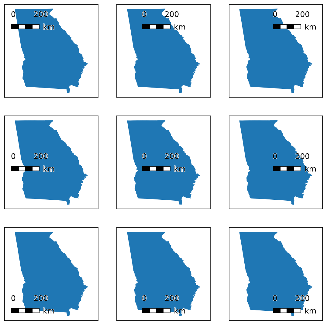
# Grid of location options
# Note that the "center" options will feel slightly off: this is because the the center of the scale bar is of the entire artist, text included, not just the bar itself
locs = ["upper left", "upper center", "upper right", "center left", "center", "center right", "lower left", "lower center", "lower right"]

fig, axs = new_map(3,3, figsize=(9,9))

for ax,l in zip(axs.flatten(), locs):
    states.query(f"NAME=='Georgia'").plot(ax=ax)
    ax.set_aspect(1, adjustable="datalim")
    scale_bar(ax=ax, size="xs", location=l, style="boxes", bar={"projection":3857,"minor_type":"none"}, labels={"style":"first_last"})

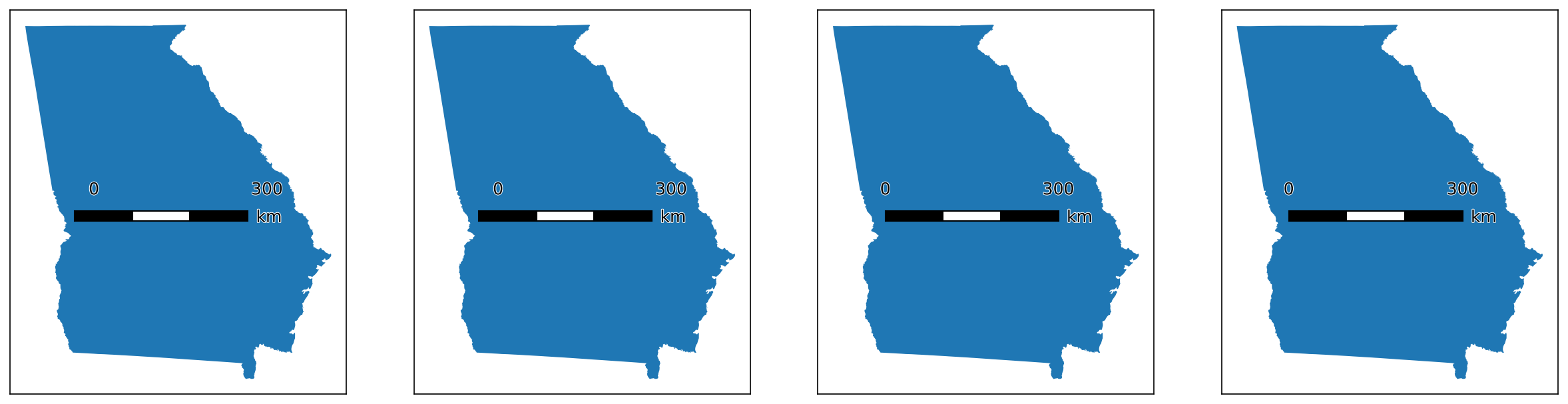
grid of plots showing possible location options

# Modifying the styles
styles = ["boxes","ticks"]

# Creating 1x2 subplots
fig, axs = new_map(1,2, figsize=(10,5))

for ax,s in zip(axs.flatten(), styles):
    states.query(f"NAME=='Georgia'").plot(ax=ax)
    ax.set_aspect(1, adjustable="datalim")
    scale_bar(ax=ax, location="center", style=s, 
            bar={"projection":3857,"minor_type":"none","length":0.5}, labels={"style":"first_last"})

two plots showing possible style options

# An example to show changing zorders
zorders = [{"plot":5,"scale":10}, {"plot":10,"scale":5}]

# Creating four subplots
fig, axs = new_map(1,2, figsize=(10,5))

for ax,z in zip(axs.flatten(), zorders):
    states.query(f"NAME=='Georgia'").plot(ax=ax, zorder=z["plot"])
    ax.set_aspect(1, adjustable="datalim")
    scale_bar(ax=ax, location="upper left", 
            bar={"projection":3857,"minor_type":"none","length":0.5}, labels={"style":"first_last"}, zorder=z["scale"])

comparison of different zorder values for the scale bar

Visible Components¶

There are three "visible" components to the scale bar. Each of these is separately customisable, but unlike the NorthArrow object, they cannot can be turned off entirely by passing a value of False to the function or during object, as each component is necessary for a ScaleBar (passing None still uses default values).

Bar¶

bar is the most important component, and has the most customisation options.

Attribute	Description	Accepts
`projection`	The coordinate reference system (CRS) that the map is in (I am considering making it a top-level variable like `style` and `location`). Projected vs Unprojected Projected reference systems are preferred; unprojected ones will be approximated to metres based on the great circle distance.	Any `pyproj` CRS value, including strings and integers, as well as the special options available per this subsection
`unit`	The unit of measurement that you want the scale bar to be in. If left blank, will be the same as the unit of measurement of the `projection`. Otherwise, will handle conversion between the two: useful if you are using a projection in metres and want to convert it to kilometers or feet. Auto-Scaling if left blank, or set to `None`, this will auto-scale meters and feet to kilometers and miles, respectively, when the axis is >5 kilometers or miles wide/tall. To disable this behavior, simply specify a value for this argument (i.e. `unit="ft"`).	See `validation.scale_bar.units_standard` for acceptable values, but the following shorthand will work: `m` for meters, `ft` for feet, `km` for kilometers, `yd` for yards, `mi` for miles, `nmi` for nautical miles
`rotation`	For rotating the scale bar an arbitrary number of degrees; useful for creating a vertically-oriented scale bar.	A number between -360 and 360
`max`	The max value of the scale bar, in the same units as `unit` (or `projection` if `unit` is None). If left blank, will be approximated based on the value of `length`.	Any positive number
`length`	The desired length of the bar in inches (for values greater than 1), or as a fraction of the axis width (for values between 0 and 1) If left blank, will be approximated as ~25% of the axis. Auto-Rounding Note that any values set here will also be rounded for convenience: so if you want a 3 inch scale bar, but that equals 91,000 kilometers, you should expect that to be rounded down to 90,000 kilometers, and your scale bar to therefore be a little less than 3 inches.	Any positive number
`height`	The desired height of the bar (cross-axis from the bar `length` regardless of orientation set by `rotation`) in inches. Note that for `ticks`, this will set the height of the `major` ticks (instead of the `minor` ones).	Any positive number
`reverse`	Whether or not to flip the order of the bar's segments; for a "typical" scale bar, that would mean the max is on the left instead of the right.	Either `True` or `False`
`major_div`	The number of "major" divisions in the bar (see minor divisions below for the difference). Note that this can only be set alongside `max`: setting it on its own will not do anything. If left blank, will be approximated based on the `length` and `max` values.	Any integer
`major_mult`	The length of a "major" division in the bar - only used when specifying the length of the bar as a multiple of major divisions and division size (see this section for details). Note that this can only be used in conjunction with `major_div`: setting it on its own will not do anything.	Any integer
`minor_div`	The number of "minor" divisions in each major division; a bar with 2 major division and 2 minor divisions will have 4 divisions in total.	Any integer, but must be greater than 1 for a minor division to be visible
`minor_type`	Controls where minor divisions will appear: If set to `none`, will not have any minor divisions, regardless of what `minor_div` is set to. If set to `first`, then only the first major division will be subdivided; the rest will be intact. If set to `all`, all major divisions will be subdivided.	Any of `none`, `first`, or `all`

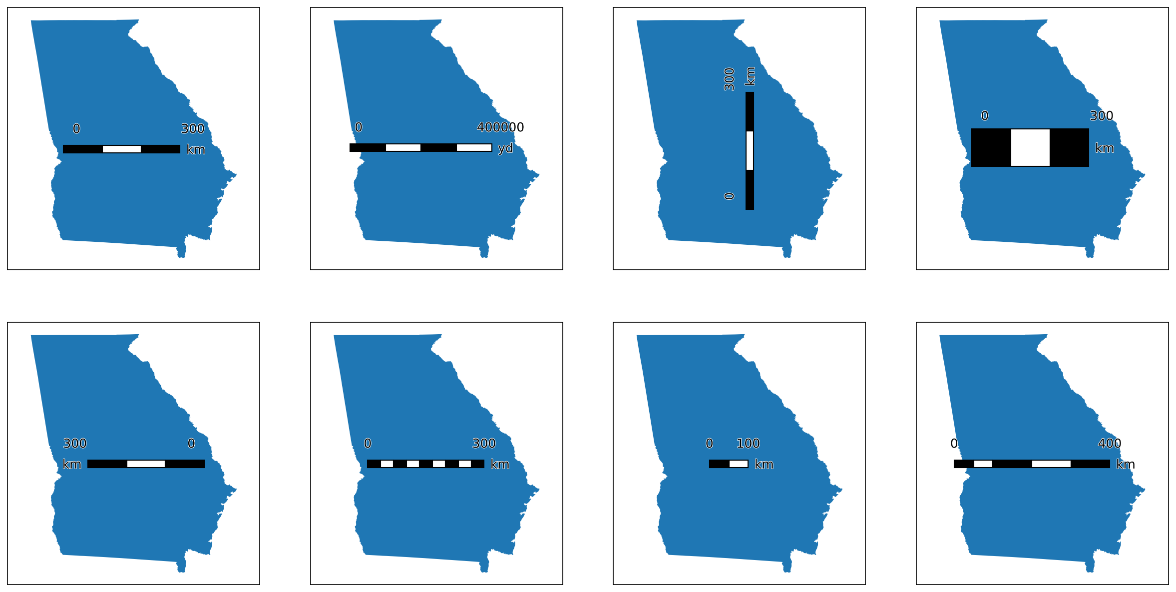
# Modifying specific elements
modifications = [
    {}, # default settings for comparison
    {"unit":"yd"}, # converting units
    {"rotation":90}, # making the bar vertical
    {"height":0.5}, # increasing the height
    {"reverse":True}, # reversing the order of the bar
    {"minor_type":"all"}, # adding minor divisions
    {"length":0.2}, # shortening the bar
    {"length":None,"max":400,"major_div":4,"minor_div":2,"minor_type":"first"}, # setting all the bar divisions
]

# Creating 2x4 subplots
fig, axs = new_map(2,4, figsize=(20,10))

for ax,m in zip(axs.flatten(), modifications):
    states.query(f"NAME=='Georgia'").plot(ax=ax)
    ax.set_aspect(1, adjustable="datalim")
    scale_bar(ax=ax, location="center", style="boxes", labels={"style":"first_last"},
            bar={"projection":3857,"minor_type":"none","length":0.5} | m) # this line just concatenates the two dictionaries together

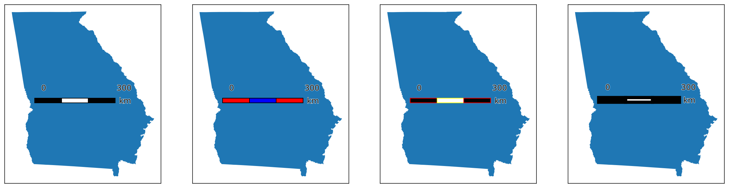
array of different visible component settings

Some additional options are also available based on the the selected style of bar:

BoxesTicks

Attribute	Description	Accepts
`facecolors`	The color(s) of the division on the bar. If a single value is passed, it will be used for all divisions. If a list is passed, it will be extended via cycling to the appropriate length (based on the number of division in the bar) if shorter, or it will be truncated, if longer.	Any `matplotlib` color
`edgecolors`	The color(s) of the edges of the divisions on the bar. If a single value is passed, it will be used for all divisions. If a list is passed, it will be extended via cycling to the appropriate length (based on the number of division in the bar) if shorter, or it will be truncated, if longer.	Any `matplotlib` color
`edgewidth`	The width of the edge of the divisions. Only a singular value may be passed.	Any positive number

# Modifying specific elements
modifications = [
    {}, # default settings for comparison
    {"facecolors":["red","blue"]}, # changing the colors of the divisions
    {"edgecolors":["red","yellow"]}, # changing the colors of the edges
    # NOTE: I do think this changes the length of the bar which I don't love, so large values not recommended (relative to plot size)
    {"edgewidth":5}, # changing the width of the edges 
]

# Creating 1x4 subplots
fig, axs = new_map(1,4, figsize=(20,5))

for ax,m in zip(axs.flatten(), modifications):
    states.query(f"NAME=='Georgia'").plot(ax=ax)
    ax.set_aspect(1, adjustable="datalim")
    scale_bar(ax=ax, location="center", style="boxes", labels={"style":"first_last"},
            bar={"projection":3857,"minor_type":"none","length":0.5} | m) # this line just concatenates the two dictionaries together

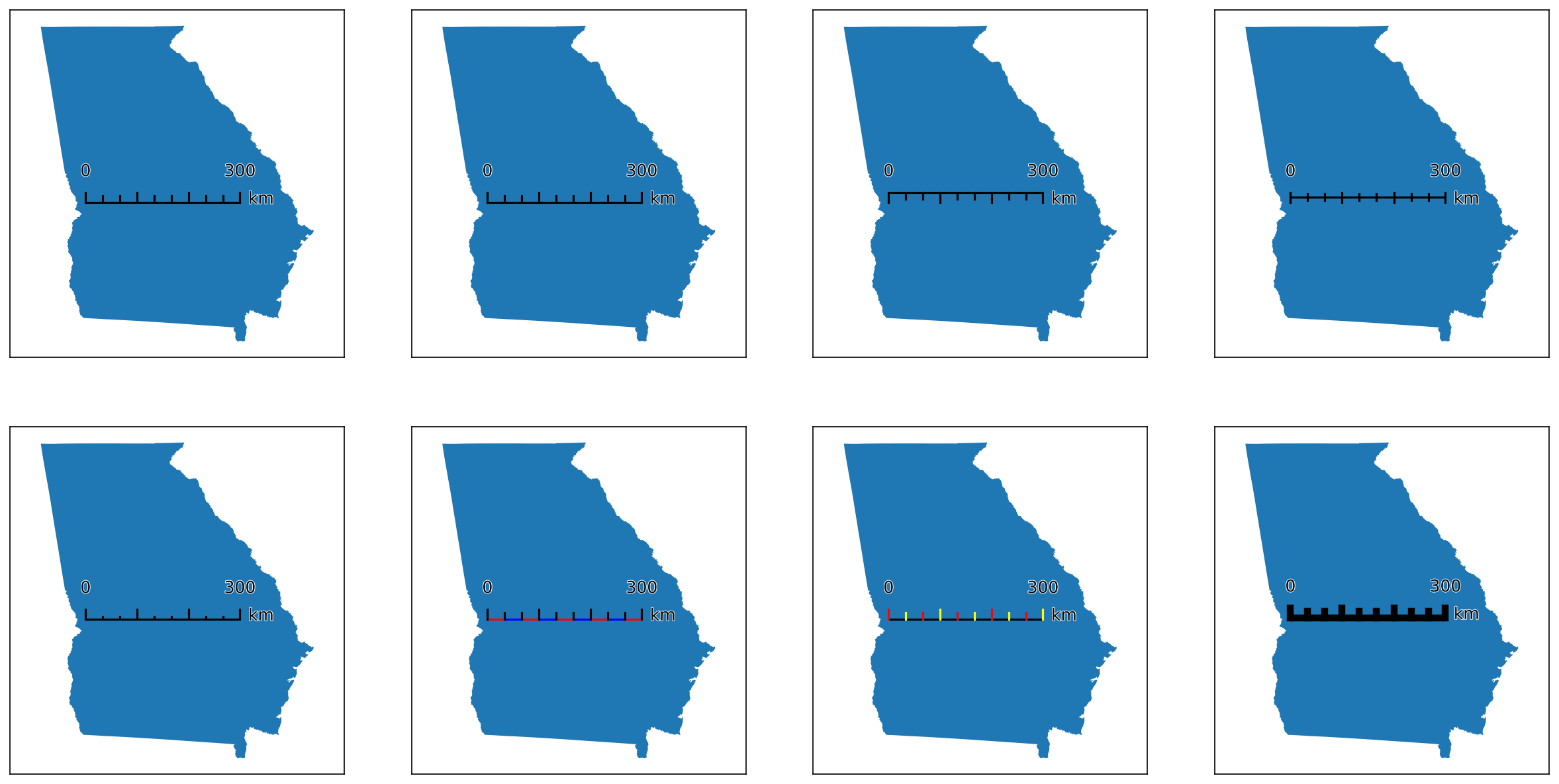
array of different visible component settings for boxes bars

Attribute	Description	Accepts
`minor_frac`	the height of the `minor` ticks, as a fraction of the height of the major ticks (set by `height`); a value of `0.5` will create minor ticks half the height of the major ticks.	Any positive number
`tick_loc`	the position of the ticks relative to the base bar.	Any of `above`, `below`, or `middle` (if ticks should intersect the bar midway)
`basecolors`	The color(s) of the segments that comprise the "base" of the scale bar. If a single value is passed, it will be used for all divisions. If a list is passed, it will be extended via cycling to the appropriate length (based on the number of division in the bar) if shorter, or it will be truncated, if longer.	Any `matplotlib` color
`tickcolors`	The color(s) of the ticks marking the scale bar. If a single value is passed, it will be used for all divisions. If a list is passed, it will be extended via cycling to the appropriate length (based on the number of division in the bar) if shorter, or it will be truncated, if longer.	Any `matplotlib` color
`tickwidth`	The width of the base bar and ticks. Only a singular value may be passed.	Any positive number

# Modifying specific elements
modifications = [
    {}, # default settings for comparison
    # Iterating through the three tick locations
    {"tick_loc":"above"},
    {"tick_loc":"below"},
    {"tick_loc":"middle"},
    # Iterating through the other settings
    {"minor_frac":0.25}, # the default value is 0.66
    {"basecolors":["red","blue"]}, # changing the colors of the divisions
    {"tickcolors":["red","yellow"]}, # changing the colors of the edges
    {"tickwidth":5}, # changing the width of the edges 
]

# Creating 2x4 subplots
fig, axs = new_map(2,4, figsize=(20,10))

for ax,m in zip(axs.flatten(), modifications):
    states.query(f"NAME=='Georgia'").plot(ax=ax)
    ax.set_aspect(1, adjustable="datalim")
    scale_bar(ax=ax, location="center", style="ticks", labels={"style":"first_last"},
            bar={"projection":3857,"minor_type":"all","length":0.5} | m) # this line just concatenates the two dictionaries together

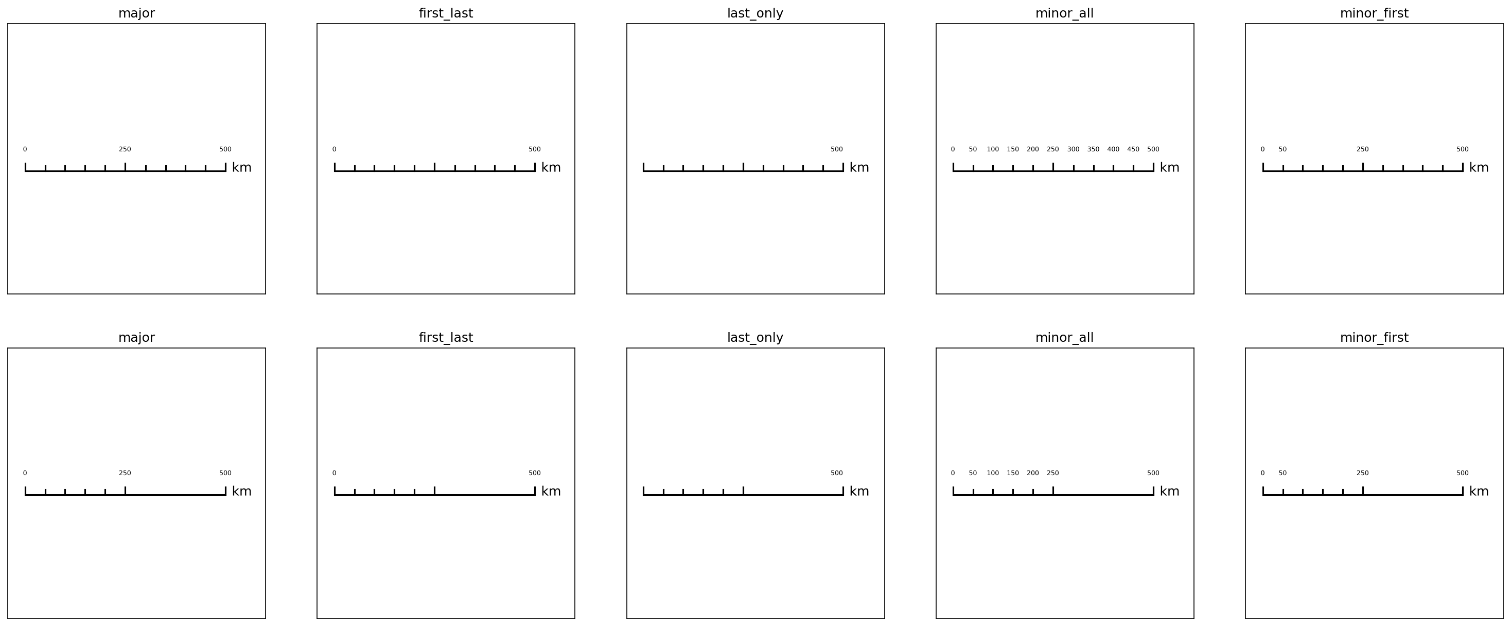
array of different visible component settings for ticks bars

Labels¶

labels modifies the text that appears on the divisions of the scale bar (i.e. not including the units text).

Attribute	Description	Accepts
`labels`	An override for the label text. Works in tandem with `style` - the number of labels provided should match the number expected based on the `style`. A value of `None` or `True` will auto-generate labels based on the `format` and `format_int` arguments. A `False` value will hide auto-generated labels.	An array of strings, `True`/`False`, or `None`
`format`	A format string that can be passed to format the auto-generated labels, if `labels` is `None`. Note: do not pass the leading semicolon (i.e. if you want to format with three decimal points, just pass `.3f`).	Valid format string; default is `.0f`
`format_int`	If `True` (default), will format "round" floats as integers, by removing their trailing decimals. If `False`, will apply the `format` string to them.	`True` or `False`
`style`	Controls which labels are placed, based on major/minor divisions. If `major`, labels will be placed on each major division, regardless of if minor divisions exist (# labels = `major_div` + 1). If `first_last`, labels will be placed on the first (0) and last major division (# labels = 2). If `last_only`, labels will be placed exclusively on the last major division (# labels = 1). If `minor_all`, labels will be placed on each major and minor division, for each minor division that exists (# labels = `major_div * minor_div + 1`). If `minor_first`, labels will be placed on each major division, and the first (and only the first) minor division (# labels = `major_div + 2`).	Any of `major`, `first_last`, `last_only`, `minor_all`, or `minor_first`
`loc`	Controls where labels are placed. If `above`, labels will be placed above the bar; if `below`, labels will be placed below.	Any of `above` or `below`
`fontsize`	The size of the text - see `matplotlib` documentation for more details..	Any float, int, or string value (such as `small` or `xx-large`)
`textcolors`	The color of the main text.	Any `matplotlib` color, as either a single value or a list to be cycled across all the text values
`fontfamily`	The appearance of the text - see `matplotlib` documentation for more details.	Any of `serif`, `sans-serif`, `cursive`, `fantasy`, or `monospace`
`fontstyle`	The appearance of the text - see `matplotlib` documentation for more details.	Any of `normal`, `italic`, or `oblique`
`fontweight`	The appearance of the text - see `matplotlib` documentation for more details.	Any of `normal`, `bold`, `heavy`, `light`, `ultrabold`, or `ultralight`
`stroke_width`	The width of the outline of the text.	Any positive number
`stroke_color`	The color of the outline of the text.	Any `matplotlib` color
`rotation`	The rotation of the text in-place, expressed in degrees. Works in tandem with `rotation_mode` (below).	Any number between -360 and 360
`rotation_mode`	Changes how the rotation of the text occurs. Recommend looking at `matplotlib`'s documentation for details.	Either `anchor` or `default`
`sep`	The amount of padding between the labels and the bar, in points.	Any positive number
`pad`	The amount of padding around the combined bar and label text, in points. Note that this is usually kept at 0, as the change is a little nuanced.	Any positive number

StylesText

# Creating 2x5 subplots
fig, axs = new_map(2,5, figsize=(25,10))

# Now we define the different label settings
modifications = [
    # Iterating through the label styles
    {"style":"major"},
    {"style":"first_last"},
    {"style":"last_only"},
    {"style":"minor_all"},
    {"style":"minor_first"},
]

# We'll first iterate through each of the two minor_types
for axc,t in zip(axs, ["all","first"]):
    for ax,m in zip(axc, modifications):
        states.query(f"NAME=='Georgia'").plot(ax=ax, color="white")
        ax.set_aspect(1, adjustable="datalim")
        scale_bar(ax=ax, location="center", style="ticks", labels={"fontsize":6} | m, 
                bar={"projection":3857,"max":500,"major_div":2,"minor_div":5,"minor_type":t})
        ax.set_title(m["style"])

array of label style options

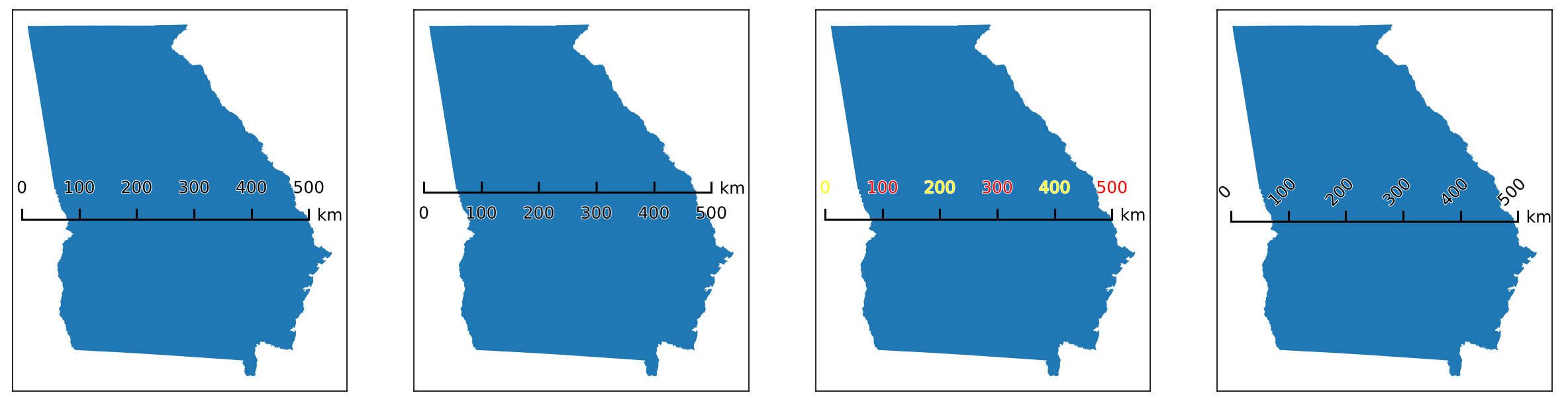
# Modifying other elements
modifications = [
    {"loc":"above"},
    {"loc":"below"},
    {"textcolors":["yellow","red"]},
    {"rotation":45}, # changing the colors of the divisions
]

# Creating 1x4 subplots
fig, axs = new_map(1,4, figsize=(20,5))

for ax,m in zip(axs.flatten(), modifications):
    states.query(f"NAME=='Georgia'").plot(ax=ax)
    ax.set_aspect(1, adjustable="datalim")
    scale_bar(ax=ax, location="center", style="ticks", labels={"style":"major"} | m, # changed the style to major here
            bar={"projection":3857,"max":500,"major_div":5,"minor_div":1,"minor_type":t})

array of text formatting options

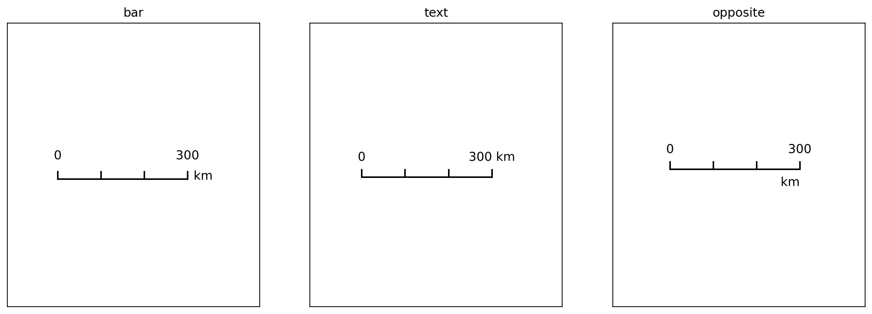
Units¶

units modifies the units label for the scale bar - it does not change the units of the scale bar itself, as that is instead controlled by bar["unit"]. By default, it uses the shorthand of the units of the scale bar (m for meters, ft for feet, etc.), but this can be manually overridden.

Attribute	Description	Accepts
`label`	An override for the default label text.	Any string
`loc`	Controls where the label is placed. If `bar`, the units labels will be placed in line with the bar (this is the default) If `text`, the label will be appended to the last label If `opposite`, will appear on the opposite side of the bar from the last label.	Any of `bar`, `text`, or `opposite`

If loc is not equal to text, you can then specify different formatting settings for the label itself:

Attribute	Description	Accepts
`fontsize`	The size of the text - see `matplotlib` documentation for more details..	Any float, int, or string value (such as `small` or `xx-large`)
`textcolor`	The color of the main text.	Any `matplotlib` color
`fontfamily`	The appearance of the text - see `matplotlib` documentation for more details.	Any of `serif`, `sans-serif`, `cursive`, `fantasy`, or `monospace`
`fontstyle`	The appearance of the text - see `matplotlib` documentation for more details.	Any of `normal`, `italic`, or `oblique`
`fontweight`	The appearance of the text - see `matplotlib` documentation for more details.	Any of `normal`, `bold`, `heavy`, `light`, `ultrabold`, or `ultralight`
`stroke_width`	The width of the outline of the text.	Any positive number
`stroke_color`	The color of the outline of the text.	Any `matplotlib` color
`rotation`	The rotation of the text in-place, expressed in degrees. Works in tandem with `rotation_mode` (below).	Any number between -360 and 360
`rotation_mode`	Changes how the rotation of the text occurs. Recommend looking at `matplotlib`'s documentation for details.	Either `anchor` or `default`

If loc is set to opposite, you can control its positioning independently:

Attribute	Description	Accepts
`sep`	The amount of padding between the units label and the bar, in points.	Any positive number
`pad`	The amount of padding around the combined bar and units label text, in points. Note that this is usually kept at 0, as the change is a little nuanced.	Any positive number

LocationsText

# This block will show the different label locations
# Creating 1x3 subplots
fig, axs = new_map(1,3, figsize=(15,5))

# Now we define the different label settings
modifications = [
    # Iterating through the label locations
    {"loc":"bar"},
    {"loc":"text"},
    {"loc":"opposite"}, # this one looks best when bar["minor_type"] = "last_only"
]

# We'll first iterate through each of the two minor_types
for ax,m in zip(axs.flatten(), modifications):
    states.query(f"NAME=='Georgia'").plot(ax=ax, color="white")
    ax.set_aspect(1, adjustable="datalim")
    scale_bar(ax=ax, location="center", style="ticks", labels={"style":"first_last"}, units=m,
                bar={"projection":3857,"max":300,"major_div":3,"minor_div":1,"minor_type":"none"})
    ax.set_title(m["loc"])

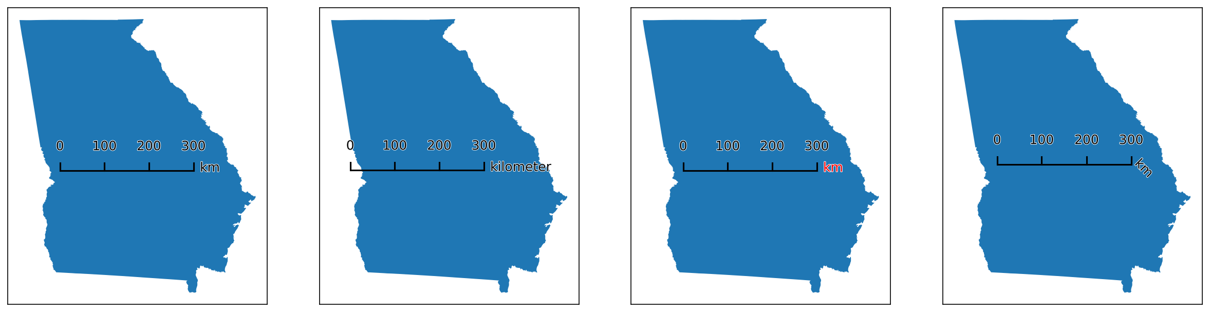
array of unit label location options

# Modifying other elements
modifications = [
    {}, # default for comparison
    {"label":"kilometer"},
    {"textcolor":"red"}, # changing the color of the units label, without affecting the other lables
    {"rotation":-45},
]

# Creating 1x4 subplots
fig, axs = new_map(1,4, figsize=(20,5))

for ax,m in zip(axs.flatten(), modifications):
    states.query(f"NAME=='Georgia'").plot(ax=ax)
    ax.set_aspect(1, adjustable="datalim")
    scale_bar(ax=ax, location="center", style="ticks", labels={"style":"major"}, units=m, # changed the style to major here
        bar={"projection":3857,"max":300,"major_div":3,"minor_div":1,"minor_type":"none"})

array of unit label formatting options

Formatting Components¶

There are two "invisible" components to the scale bar - so called because they are mainly there to help alter the position or formatting of the components, but are not directly tied to an individual component.

Text¶

text is a shorthand way of changing shared settings for the label and units together. This is useful, for example, if you want to change the fontsize, color, or family for both components, without having to set each setting twice.

Attribute	Description	Accepts
`fontsize`	The size of the text - see `matplotlib` documentation for more details..	Any float, int, or string value (such as `small` or `xx-large`)
`textcolor`	The color of the main text. Unlike the relevant setting in `label`, will only accept a single value to be used for all the text colors at once.	Any `matplotlib` color
`fontfamily`	The appearance of the text - see `matplotlib` documentation for more details.	Any of `serif`, `sans-serif`, `cursive`, `fantasy`, or `monospace`
`fontstyle`	The appearance of the text - see `matplotlib` documentation for more details.	Any of `normal`, `italic`, or `oblique`
`fontweight`	The appearance of the text - see `matplotlib` documentation for more details.	Any of `normal`, `bold`, `heavy`, `light`, `ultrabold`, or `ultralight`
`stroke_width`	The width of the outline of the text.	Any positive number
`stroke_color`	The color of the outline of the text.	Any `matplotlib` color
`rotation`	The rotation of the text in-place, expressed in degrees. Works in tandem with `rotation_mode` (below).	Any number between -360 and 360
`rotation_mode`	Changes how the rotation of the text occurs. Recommend looking at `matplotlib`'s documentation for details.	Either `anchor` or `default`

# Modifying specific elements
modifications = [
    {}, # default settings
    {"fontsize": 16}, # increased size
    {"fontweight": "bold"}, # different weight
    {"stroke_color": "black", "stroke_width":3, "textcolor": "white"}, # changing the mode, not a great example
]

# Creating four subplots
fig, axs = new_map(1,4, figsize=(20,5))

for ax,m in zip(axs.flatten(), modifications):
    states.query(f"NAME=='Georgia'").plot(ax=ax)
    ax.set_aspect(1, adjustable="datalim")
    scale_bar(ax=ax, location="center", style="ticks", labels={"style":"major"}, text=m,
            bar={"projection":3857,"max":300,"major_div":3,"minor_div":1,"minor_type":"none"})

array of text formatting options

AOB¶

aob customizes the AnchoredOffsetBox object that handles the positioning of the final scale bar object with respect to the plot. Note that facecolor, edgecolor, and alpha are non-standard options.

Attribute	Description	Accepts
`facecolor`	The color of the `AnchoredOffsetBox` patch.	Any `matplotlib` color
`edgecolor`	The color of the edge of the `AnchoredOffsetBox` patch.	Any `matplotlib` color
`alpha`	The transparency of the `AnchoredOffsetBox` patch.	Any `matplotlib` color
`pad`	The amount of padding around the north arrow, defining the edges of the `AnchoredOffsetBox`. Expressed as a fraction of the fontsize specified in `prop`.	Any positive number
`borderpad`	The amount of padding between the `AnchoredOffsetBox` and the `bbox_to_anchor`, if one is specified. Expressed as a fraction of the fontsize specified in `prop`.	Any positive number
`prop`	A reference fontsize used to define the paddings of `pad` and `borderpad`.	Any valid fontsize input
`frameon`	Whether or not to draw a frame around the box.	Either `True` or `False`
`bbox_to_anchor` and `bbox_transform`	Used to customize the placement of the `AnchoredOffsetBox`.	See Tips and Tricks section for details

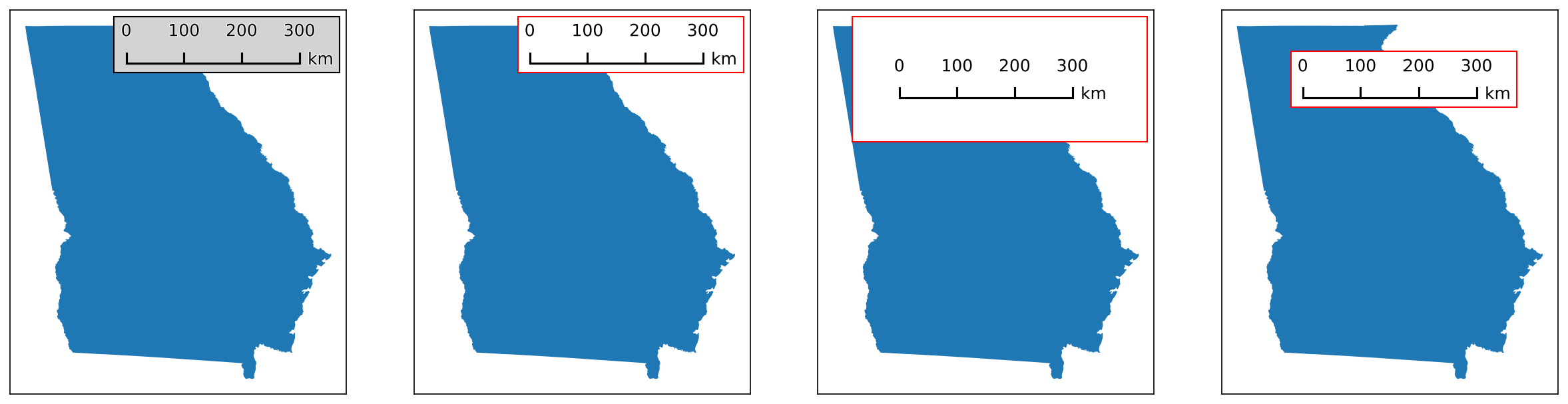
# Modifying specific elements

modifications = [
    {"facecolor": "lightgrey"}, # different facecolor
    {"edgecolor": "red"}, # different edgecolor; note that this automatically sets the facecolor to white
    # these two show the difference between pad and borderpad
    {"edgecolor": "red", "pad": 3}, # increased pad
    {"edgecolor": "red", "borderpad": 3}, # increased borderpad, which is "invisible" relative to where the edge is
]

# Creating four subplots
fig, axs = new_map(1,4, figsize=(20,5))

for ax,m in zip(axs.flatten(), modifications):
    states.query(f"NAME=='Georgia'").plot(ax=ax)
    ax.set_aspect(1, adjustable="datalim")
    scale_bar(ax=ax, location="upper right", style="ticks", labels={"style":"major"}, aob=m, # using location="upper right" to illustrate borderpad
            bar={"projection":3857,"max":300,"major_div":3,"minor_div":1,"minor_type":"none"})

array of AOB formatting options

Tips and Tricks¶

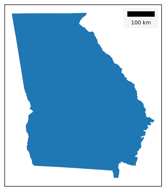
Recreating `matplotlib-scalebar`¶

The initial inspiration for creating this package was matplotlib-scalebar, which has not been updated in a while, and was generally found to be insufficient for geographic needs in particular. However, for those who want to recreate the look of the scalebars created by the package, there is a trick for doing so: if label["style"]=="last_only" and major_div==1 and minor_div==1, then the label will be drawn centered underneath the 1-div bar.

fig, ax = new_map(1,1, figsize=(5,5))

# Plotting the a state
states.query(f"NAME=='Georgia'").plot(ax=ax)

# Setting up the scale bar
scale_bar(ax=ax, location="upper right", style="boxes",
        bar={"projection":3857,"max":100,"major_div":1,"minor_div":1,"minor_type":"none"},
        labels={"style":"last_only","loc":"below","fontsize":8}, units={"loc":"text"},
        aob={"facecolor":"whitesmoke","edgecolor":"none","pad":0.5,"borderpad":0.5})

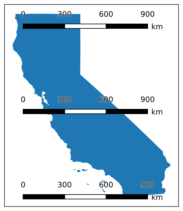
a recreation of matplotlib-scalebar

Setting Size¶

While the scale bar can nominally have its size changed by changing the length attribute, doing so doesn't change the other, related components, such as the sizes of the text, the the box dimensions, the stroke widths, and so on.

However, given that there are standardized paper sizes that most graphics are made towards, a size parameter is available that will select pre-configured default values that approximate what looks best at each size. The parameter takes in only one input, which is the size tier you want:

xsmall or xs for A8 paper, ~2 to 3 inches
small or sm for A6 paper, ~4 to 6 inches
medium or md for A4 or letter paper, ~8 to 11 inches
large or lg for A2 paper, ~16 to 24 inches
xlarge or xl for A0 paper, ~33 to 48 inches

These default values can be seen in defaults/scale_bar.py.

# For reference, this is 5 inches x 10 inches
fig, ax = new_map(1,1, figsize=(5,10))

# Plotting the a state
states.query(f"NAME=='California'").plot(ax=ax)

# Visualizing three different sizes at various positions
for s,l in zip(["sm","md","lg"], ["upper center", "center", "lower center"]):
    scale_bar(ax=ax, size=s, location=l, style="boxes", labels={"style":"major"}, 
            bar={"projection":3857,"max":900,"major_div":3,"minor_div":1,"minor_type":"none"})

# No need to reset sizes - the size= parameter handles it per-call

comparison of default scale bar sizes

Placing Scale Bars Outside of Axis¶

Sometimes it is more desireable to place the scale bar outside of the plot entirely, which can be accomplished using bbox_to_anchor and bbox_transform from the aobcomponent settings. This works the same way it does for matplotlib.pyplot.legend.

fig, ax = new_map()

states.query("NAME=='Georgia'").plot(ax=ax)

scale_bar(ax=ax, location="upper center", style="boxes", labels={"style":"major"}, 
            bar={"projection":3857,"max":500,"major_div":5,"minor_div":1,"minor_type":"none"}, 
            aob={"bbox_to_anchor":(0.5,-0.01), "bbox_transform":ax.transAxes})

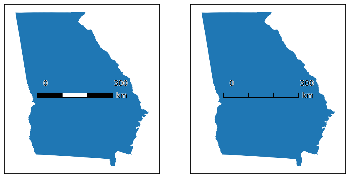
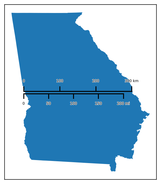
placement of the scale bar outside of the main axis

Dual Scale Bars¶

One common form for scale bars is to present two of them side-by-side, with different units of measurement (such as kilometres and miles). This can be accomplished in two ways:

dual_bars()Manually

Using the function dual_bars() will recreate the steps outlined in Manually automatically, though with more limited customization between the two bars: you can only change the units, bar_max, bar_length, major_div, and minor_div of the bars; all formatting elements must be the same.

Warning

This function is experimental, and is particularly prone to breaking when rotation is set to a value other than 0 - if people give feedback that it is useful, I will spend time cleaning it up!

# Using dual_bars()
from matplotlib_map_utils import dual_bars

fig, ax = new_map(1,1, figsize=(5,5))
_ = states.query("NAME=='Georgia'").to_crs(3520).plot(ax=ax)

# Note that this handles the flipping of the ticks and labels automatically!
dual_bars(ax=ax, draw=True, style="ticks", location="center", 
        # For these settings, the first item in the list will apply to the top bar, and the second to the bottom
        units_dual=["km","mi"], bar_maxes=[300,200], major_divs=[3,4], minor_divs=[1,1], # you could set bar_length=[x,y] here too
        # These settings are shared among all the bars
        bar={"projection":3520,"rotation":0,"reverse":False,"minor_type":"none"},
        labels={"style":"major"},
        units={"loc":"text"}, 
        text={"stroke_width":1,"stroke_color":"white","fontsize":"xx-small"},
        # These settings are for the V/HPacker (see the manual example)
        sep=1.5, pad=0)

dual scale bars via the included function

Create two bars using the scale_bar() function with draw=False and return_aob=False. Each function will return an OffsetImage object, which can be placed in a VPacker or HPacker, and the placed in a AnchoredOffsetBox to assist with positioning. Note that any settings passed to aob will be ignored!

# Manual version
import matplotlib.offsetbox

fig, ax = new_map(1,1, figsize=(5,5))
_ = states.query("NAME=='Georgia'").to_crs(3520).plot(ax=ax)

# First the bar showing kilomtres
km = scale_bar(ax=ax, draw=False, return_aob=False, style="ticks", location="center",
                bar={"projection":3520,"unit":"km","max":300,"major_div":3,"minor_div":1,
                            "rotation":0,"reverse":False,"minor_type":"none"},
                labels={"style":"major"},
                units={"loc":"text"}, 
                text={"stroke_width":1,"stroke_color":"white","fontsize":"xx-small"})

# Then the bar showing miles
# Note that I have to MANUALLY change the location of the ticks and the lables
mi = scale_bar(ax=ax, draw=False, return_aob=False, style="ticks", location="center",
                bar={"projection":3520,"unit":"mi","max":200,"major_div":4,"minor_div":1,
                            "rotation":0,"reverse":False,"minor_type":"none","tick_loc":"below"},
                labels={"style":"major","loc":"below"},
                units={"loc":"text"}, 
                text={"stroke_width":1,"stroke_color":"white","fontsize":"xx-small"})

# Now, placing each OffsetImage inside of a VPacker
pack = matplotlib.offsetbox.VPacker(children=[km,mi], align="left", pad=0, sep=1.5)
# And placing that into an AnchoredOffsetBox
aob = matplotlib.offsetbox.AnchoredOffsetbox(loc="center", child=pack, frameon=False)
# And drawing it onto the axis
_ = ax.add_artist(aob)

dual scale bars via manual placement

Accessing Artists¶

Unlike the North Arrow, the the rotation option is meant to affect all of the subcomponents: boxes/ticks and labels. As far as I can tell, this is not possible with an AnchoredOffsetBox (which contains all the subcomponents) placed inside of an AuxTransformBox (which can apply a rotation transformation) - I tried many times to debug this, if you know how to make it work then let me know.

Instead, I render the final box, pre-rotation, as an Image using matplotlib's buffer_rgba() on a temporary figure I constructed. This flattens everything, returning just the array of Image values that I then use to create an OffsetImage(), which is what is ultimately returned. See the function render_as_image() in core.scale_bar.py if you are interested to see how it works.

Scale Bars

Set-Up¶

Creating a Scale Bar¶

Using the scale_bar() function¶

Using the ScaleBar class¶

Re-using Objects¶

Updating Objects¶

Customizing the Scale Bar¶

Specifying Length¶

Primary Settings¶

Visible Components¶

Bar¶

Labels¶

Units¶

Formatting Components¶

Text¶

AOB¶

Tips and Tricks¶

Recreating matplotlib-scalebar¶

Setting Size¶

Placing Scale Bars Outside of Axis¶

Dual Scale Bars¶

Accessing Artists¶

Using the `scale_bar()` function¶

Using the `ScaleBar` class¶

Recreating `matplotlib-scalebar`¶