North Arrows
This guide is structured like a tutorial, in order to showcase the various options and methods available; if you would like to follow along, a few additional packages and set-up steps are required:
Set-Up
# Packages used by this tutorial
import geopandas # manipulating geographic data
import numpy # creating arrays
import pygris # easily acquiring shapefiles from the US Census
import matplotlib.pyplot # visualization

# Downloading the state-level dataset from pygris
states = pygris.states(cb=True, year=2022, cache=False).to_crs(3857)

# This is just a function to create a new, blank map with matplotlib, with our default settings
def new_map(rows=1, cols=1, figsize=(5,5), dpi=150, ticks=False):
    # Creating the plot(s)
    fig, ax = matplotlib.pyplot.subplots(rows,cols, figsize=figsize, dpi=dpi)
    # Turning off the x and y axis ticks
    if ticks==False:
        if rows > 1 or cols > 1:
            for a in ax.flatten():
                a.set_xticks([])
                a.set_yticks([])
        else:
            ax.set_xticks([])
            ax.set_yticks([])
    # Returning the fig and ax
    return fig, ax
The above is only necessary for this specific tutorial; below, we import the main elements related to north arrows:
Creating a North Arrow
Using the north_arrow() function
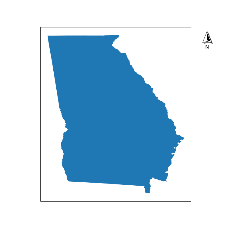
The quickest and easiest way to add a north arrow to a single plot is using the north_arrow() function. This will automatically create the artist and apply it to the supplied axis.
# Setting up a plot
fig, ax = new_map()

# Plotting a state (Georgia)
states.query("NAME=='Georgia'").plot(ax=ax)

# Adding a north arrow to the upper-right corner of the axis, without any rotation (see Rotation under Formatting Components for details)
north_arrow(ax=ax, location="upper right", rotation={"degrees":0})
![]()
Using the NorthArrow class
Alternatively, a NorthArrow class (based on matplotlib.artist.Artist) is also provided that allows the same arrow to be rendered like so:
# Setting up a plot
fig, ax = new_map()

# Plotting a state (Georgia)
states.query("NAME=='Georgia'").plot(ax=ax)

# Creating a NorthArrow object that we want to place in the upper-right corner of the axis,
# without any rotation (see Rotation under Formatting Components for details)
# Note that here, we do not specify the axis
na = NorthArrow(location="upper right", rotation={"degrees":0})

# The NorthArrow can then be added using add_artist(), which calls its built-in draw() function:
ax.add_artist(na)
![]()
Re-using Objects
The benefit of the NorthArrow object is that it can be re-used across multiple plots without copy-pasting the function call. This is particularly beneficial for highly-customized arrows: you can simply set it up once, and then add it to each axis you want.
The caveat to this is that instead of using ax.add_artist(NorthArrow), you have to use ax.add_artist(NorthArrow.copy()), as matplotlib does not let you add the same artist to multiple axes, so you have to add a copy of the artist.
Here, we try and re-use the na artist we created above, which has already been applied to the plot of Georgia
# Setting up a plot
fig, ax = new_map()

# Plotting a new state (Texas)
states.query("NAME=='Texas'").plot(ax=ax)

# Trying to re-use the same artist - this will throw an error
ax.add_artist(na)
Returns:
Now, we're starting from scratch:
# Setting up plots for both Georgia and Texas
ga_fig, ga_ax = new_map()
tx_fig, tx_ax = new_map()

# Plotting each state
states.query("NAME=='Georgia'").plot(ax=ga_ax)
states.query("NAME=='Texas'").plot(ax=tx_ax)

# Setting up the north arrow artist
na = NorthArrow(location="upper right", rotation={"degrees":0})

# Applying the artist to each plot
# Note we have to call .copy() EACH TIME
ga_ax.add_artist(na.copy())
tx_ax.add_artist(na.copy())
Returns:
Updating Objects
The customization options of the NorthArrow can be accessed using dot notation (like na.base, na.label, etc.). They can also be updated from this dot notation by passing a valid style dictionary (see next section for details).
Returns:
Returns:
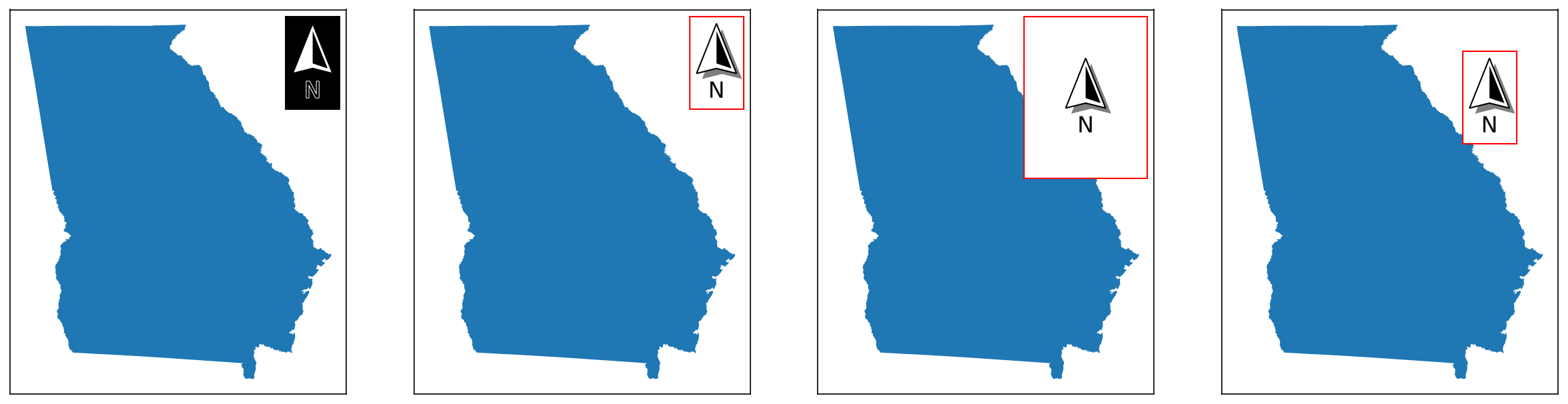
This means you can update the properties of the created class while it is in use, in case you want small changes made in between iterations:
shapes = ["Texas","Georgia","California","Louisiana"]
labels = ["First","Second","Third","Fourth"]

# Creating the initial arrow
na = NorthArrow(location="upper right", rotation={"degrees":0})

# Creating four subplots
fig, axs = new_map(1,4, figsize=(20,5))

for ax,s,l in zip(axs.flatten(), shapes, labels):
    states.query(f"NAME=='{s}'").plot(ax=ax)
    ax.set_aspect(1, adjustable="datalim")
    na.label = {"text":l}
    ax.add_artist(na.copy())
![]()
Though for this specific example, you could accomplish the same with the north_arrow() function just as (more?) easily
shapes = ["Texas","Georgia","California","Louisiana"]
labels = ["First","Second","Third","Fourth"]

# Creating four subplots
fig, axs = new_map(1,4, figsize=(20,5))

for ax,s,l in zip(axs.flatten(), shapes, labels):
    states.query(f"NAME=='{s}'").plot(ax=ax)
    ax.set_aspect(1, adjustable="datalim")
    north_arrow(ax=ax, location="upper right", label={"text":l}, rotation={"degrees":0})
![]()
Customizing the North Arrow
Both the functional and object-oriented approach use the same primitive style dictionaries, so you can treat the following information as valid for both.
Primary Settings
There are three primary settings that must be supplied each time a north arrow is created:
| Attribute | Description | Accepts |
|---|---|---|
location |
Where the arrow will be placed relative to the plot. | Any options accepted by matplotlib for legend placement ("upper right", "center", "lower left", etc., see loc in the matplotlib.pyplot.legend documentation) |
scale |
The desired size of the north arrow's height, in inches; the default is whatever size is set by the size parameter (see Tips and Tricks section). |
Any positive number |
zorder |
(new as of v3.1.0) The zorder of the final north arrow artist, which can be used to bring the artist forward / place it behind other axis artists. |
Any number; default value is 99 |
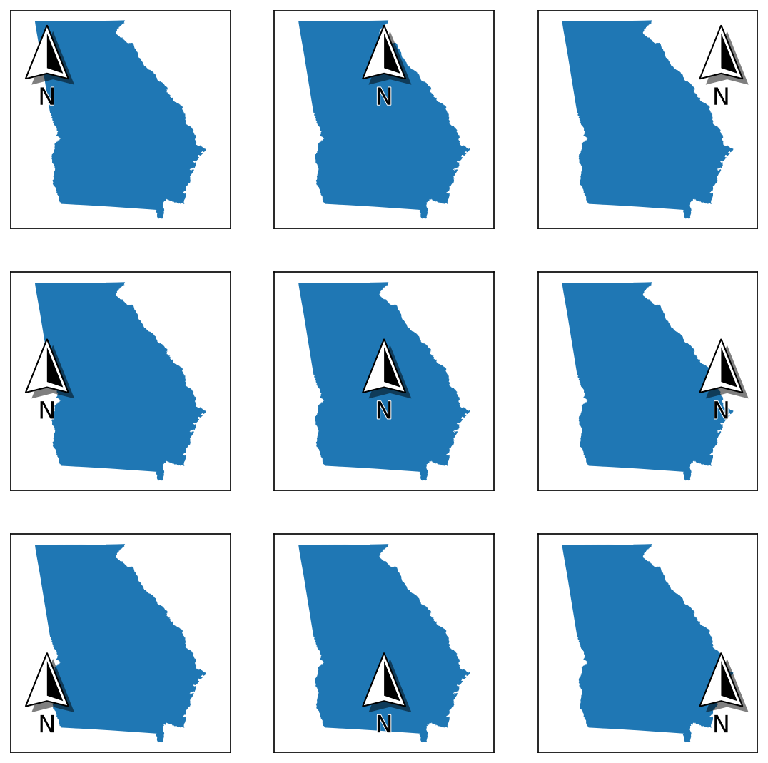
# Grid of location options
locs = ["upper left", "upper center", "upper right", "center left", "center", "center right", "lower left", "lower center", "lower right"]

fig, axs = new_map(3,3, figsize=(9,9))

for ax,l in zip(axs.flatten(), locs):
    states.query(f"NAME=='Georgia'").plot(ax=ax)
    ax.set_aspect(1, adjustable="datalim")
    north_arrow(ax=ax, location=l, rotation={"degrees":0})
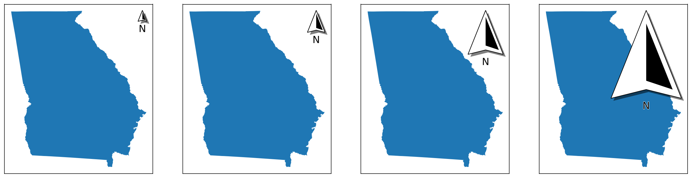
# Modifying the scale
# Recommend looking at the "Setting Size" section of "Tips and Tricks" for another way to do this!
scales = [0.25, 0.5, 1, 2]

# Creating four subplots
fig, axs = new_map(1,4, figsize=(20,5))

for ax,s in zip(axs.flatten(), scales):
    states.query(f"NAME=='Georgia'").plot(ax=ax)
    ax.set_aspect(1, adjustable="datalim")
    north_arrow(ax=ax, location="upper right", rotation={"degrees":0}, scale=s)
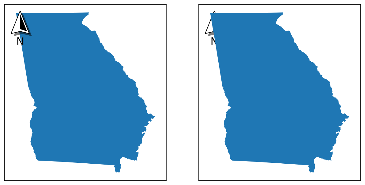
# An example to show changing zorders
zorders = [{"plot":5,"arrow":10}, {"plot":10,"arrow":5}]

# Creating four subplots
fig, axs = new_map(1,2, figsize=(10,5))

for ax,z in zip(axs.flatten(), zorders):
    states.query(f"NAME=='Georgia'").plot(ax=ax, zorder=z["plot"])
    ax.set_aspect(1, adjustable="datalim")
    north_arrow(ax=ax, location="upper left", rotation={"degrees":0}, zorder=z["arrow"])
Visible Components
There are four "visible" components to the north arrow. Each of these is separately customisable, and can be turned off entirely by passing a value of False to the function or object creation (passing None uses default values).
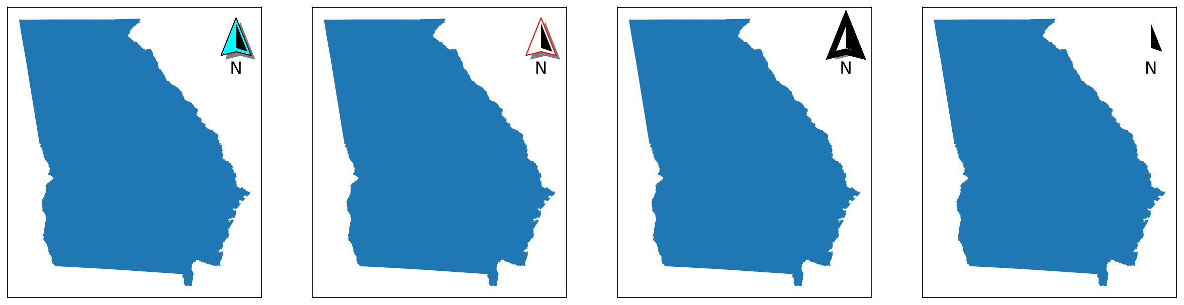
Base
base is the bottom-most visible layer and the most important component.
| Attribute | Description | Accepts |
|---|---|---|
coords |
The coordinates used to draw the shape of the base itself. Each coordinate exists on a plane from 0 to 1 in two dimensions ([0,0] being bottom-left and [1,1] being top-right, in the format [x,y]), and is multiplied by scale to get its corresponding size in inches. |
A numpy.array of two-element tuples |
facecolor |
The color of the main base patch. | Any matplotlib color |
edgecolor |
The color of the edge of the base patch. | Any matplotlib color |
linewidth |
The width of the edge of the base patch. | Any positive number |
zorder |
The drawing order of the base patch. Recommended to be a lower number than the fancy patch. Is relative to the other artists that comprise the north arrow (label, fancy), NOT to the overall plot. | Any positive number |
# Modifying specific elements
modifications = [
    {"facecolor":"cyan"}, # changing the color
    {"edgecolor":"red"}, # changing the color
    {"linewidth":6}, # changing the stroke
    False # hiding it entirely - note that the shadow is hidden here too, as it is dependent on the base artist for visibility
]

# Creating four subplots
fig, axs = new_map(1,4, figsize=(20,5))

for ax,m in zip(axs.flatten(), modifications):
    states.query(f"NAME=='Georgia'").plot(ax=ax)
    ax.set_aspect(1, adjustable="datalim")
    north_arrow(ax=ax, location="upper right", rotation={"degrees":0}, base=m)
Fancy
fancy is the half-shape patch on top of the base (in the examples above, it appears as black).
| Attribute | Description | Accepts |
|---|---|---|
coords |
The coordinates used to draw the shape of the patch itself | See the same option on the base component for details (above) |
facecolor |
The color of the patch. | Any matplotlib color |
zorder |
The drawing order of the patch. Recommended to be a higher number than the base patch. Is relative to the other artists that comprise the north arrow (label, base), NOT to the overall plot. |
Any positive number |
# Modifying specific elements
modifications = [
    True, # normal patch
    {"coords":numpy.array([(0.50, 0.85), (0.35, 0.50), (0.50, 0.55), (0.65, 0.50), (0.50, 0.85)])}, # changing the shape
    {"facecolor":"blue"}, # changing the color
    False # hiding it entirely
]

# Creating four subplots
fig, axs = new_map(1,4, figsize=(20,5))

for ax,m in zip(axs.flatten(), modifications):
    states.query(f"NAME=='Georgia'").plot(ax=ax)
    ax.set_aspect(1, adjustable="datalim")
    north_arrow(ax=ax, location="upper right", rotation={"degrees":0}, fancy=m)

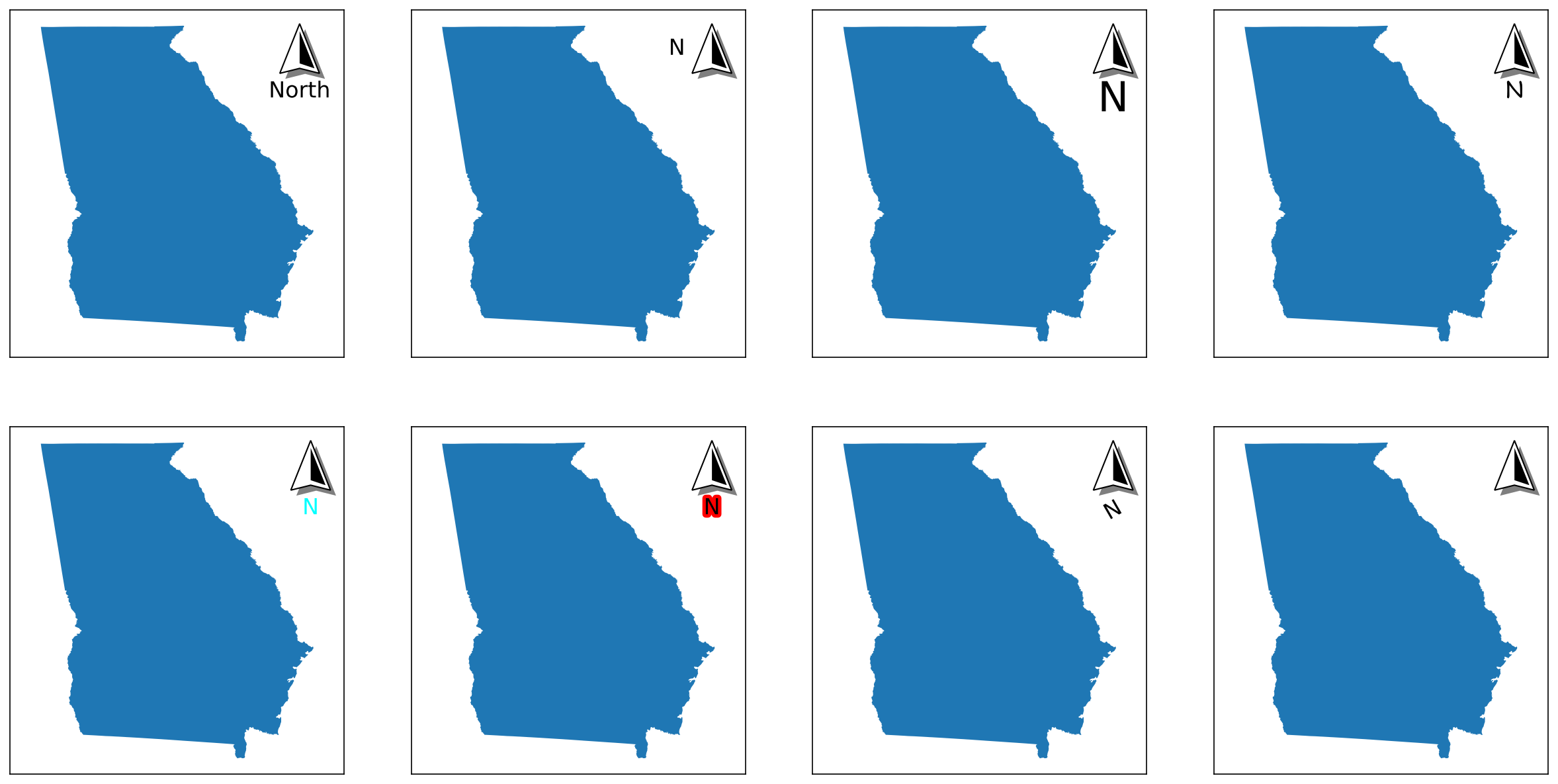
Label
label is the text that appears appears around the arrow.
| Attribute | Description | Accepts |
|---|---|---|
text |
The text that will be displayed. | Any string |
position |
The position of the text relative to the arrow itself. | Any of top, bottom, left, or right |
ha |
How the text is positioned horizontally - see matplotlib documentation for more details. |
Any of left, center, or right |
va |
How the text is positioned vertically - see matplotlib documentation for more details. |
Any of baseline, bottom, center, center_baseline, or top |
fontsize |
The size of the text - see matplotlib documentation for more details. |
Any number, or a string such as small or xx-large |
fontfamily |
The appearance of the text - see matplotlib documentation for more details. |
Any of serif, sans-serif, cursive, fantasy, or monospace |
fontstyle |
The appearance of the text - see matplotlib documentation for more details. |
Any of normal, italic, or oblique |
color |
The color of the main text. | Any matplotlib color |
fontweight |
The appearance of the text - see matplotlib documentation for more details. |
Any of normal, bold, heavy, light, ultrabold, or ultralight |
stroke_width |
The width of the outline of the text | Any positive number |
stroke_color |
The color of the outline of the text | Any matplotlib color |
rotation |
The rotation of the text centrally. Note that this works differently than the rotation of the arrow itself (see the appropriate section under Formatting Components) |
Any number |
zorder |
The drawing order of the text patch, relative to the other artists that comprise the north arrow (base, fancy), NOT to the overall plot. | Any number |
# Modifying specific elements
modifications = [
    {"text": "North"}, # changing the text
    {"position": "left"}, # changing the position
    {"fontsize": 30}, # changing the size
    {"fontfamily": "cursive"}, # changing the family
    {"color": "cyan"}, # changing the color of the text
    {"stroke_width": 5, "stroke_color": "red"}, # changing the stroke size and color
    {"rotation": 30}, # changing the rotation
    False # hiding it entirely
]

# Creating eight subplots
fig, axs = new_map(2,4, figsize=(20,10))

for ax,m in zip(axs.flatten(), modifications):
    states.query(f"NAME=='Georgia'").plot(ax=ax)
    ax.set_aspect(1, adjustable="datalim")
    north_arrow(ax=ax, location="upper right", rotation={"degrees":0}, label=m)
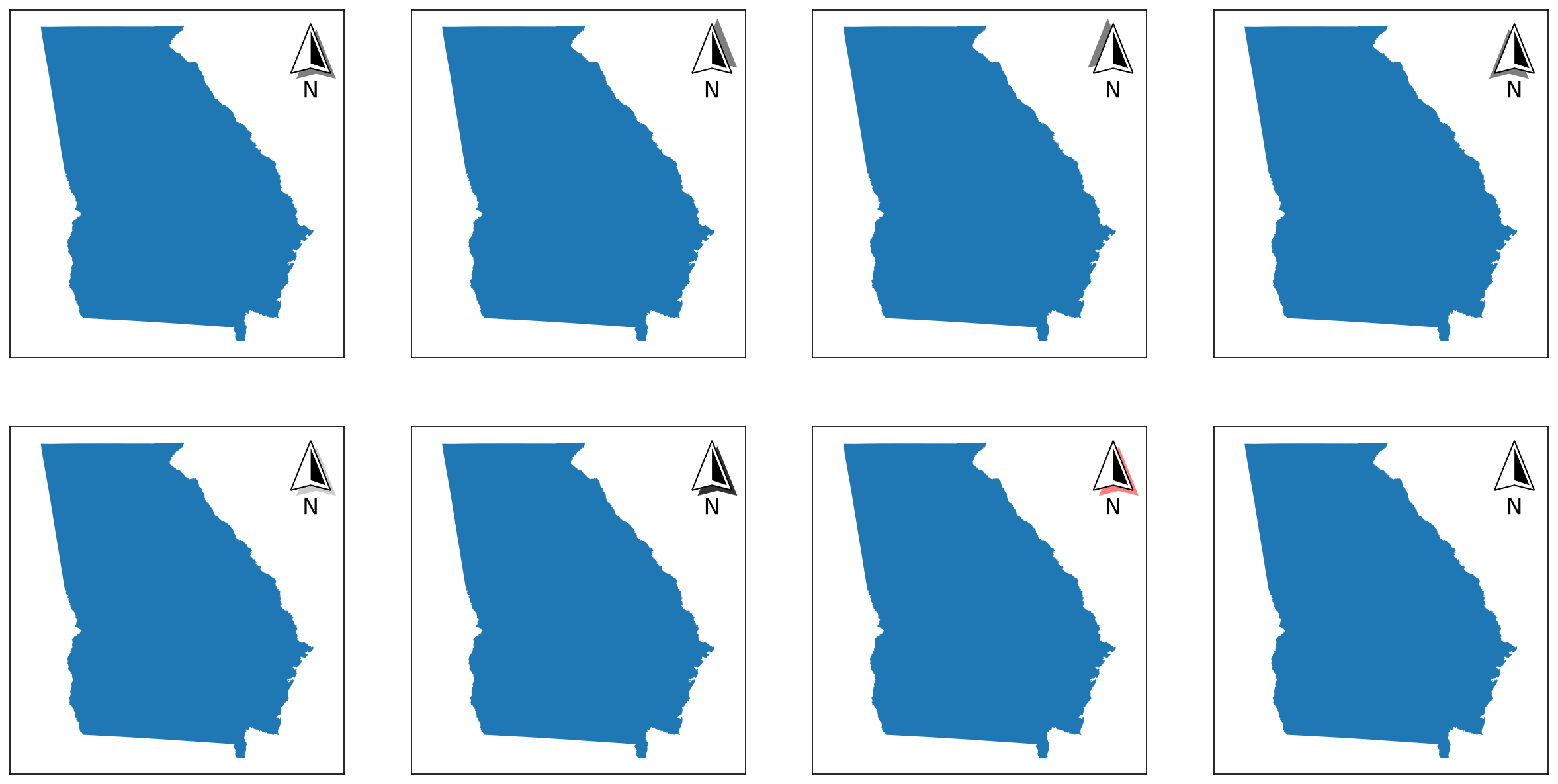
Shadow
shadow is the path effect on the base patch that creates the shadow effect - it is applied using matplotlib.patheffects.withSimplePatchShadow.
| Attribute | Description | Accepts |
|---|---|---|
offset |
Where the shadow appears relative to the base patch. | A tuple of coordinates in the order `(x,y); each coordinate can be either a float or an integer |
alpha |
The transparency of the shadow patch. | A number between 0 and 1 |
shadow_rgbFace |
The color of the shadow patch. | Any matplotlib color value |
# Modifying specific elements
modifications = [
    {"offset": (4, -4)}, # changing the offset
    {"offset": (4, 4)}, # changing the offset
    {"offset": (-4, 4)}, # changing the offset
    {"offset": (-4, -4)}, # changing the offset
    {"alpha": 0.2}, # changing the transparency
    {"alpha": 0.8}, # changing the transparency
    {"shadow_rgbFace": "red"}, # changing the color
    False # hiding it entirely
]

# Creating eight subplots
fig, axs = new_map(2,4, figsize=(20,10))

for ax,m in zip(axs.flatten(), modifications):
    states.query(f"NAME=='Georgia'").plot(ax=ax)
    ax.set_aspect(1, adjustable="datalim")
    north_arrow(ax=ax, location="upper right", rotation={"degrees":0}, shadow=m)
Formatting Components
There are three "invisible" components to the north arrow - so called because they are mainly there to help position the arrow and its individual components. Unlike the "visible" components, these cannot be turned off, but they are still separately customisable.
Pack
pack customizes the HPacker or VPacker object that handles the positioning of the label relative to the base patch (and fancy patch if it is included). Whether or not it is an HPacker or VPacker is used is dependent on the position option from the label, but the settings are the same for both.
| Attribute | Description | Accepts |
|---|---|---|
offset |
Where the shadow appears relative to the base patch. | A tuple of coordinates in the order `(x,y); each coordinate can be either a float or an integer |
alpha |
The transparency of the shadow patch. | A number between 0 and 1 |
shadow_rgbFace |
The color of the shadow patch. | Any matplotlib color value |
| sep | The amount of spacing to have between the elements, in points. | Any positive number |
| align | How each element is aligned. | Any of top, bottom, left, right, center, or baseline |
| pad | The amount of padding around the box, in points. Note that this is usually kept at 0, and controlled instead using the aob settings (below). | Any positive number |
| width and height | The dimensions of the box, in pixels. Kept as None for most circumstances so calculated manually. | Any positive number |
| mode | How the elements are packed within the box; see documentation for HPacker and VPacker as to how each mode works. | Any of fixed, expand, or equal; *default is fixed. |
# Modifying specific elements
modifications = [
    None, # default settings
    {"sep": 15}, # increased separation between items
    {"align": "left"}, # changing the alignment of items
    {"width": 100, "height": 200, "mode": "expand"}, # changing the mode, not a great example
]

# Creating four subplots
fig, axs = new_map(1,4, figsize=(20,5))

for ax,m in zip(axs.flatten(), modifications):
    states.query(f"NAME=='Georgia'").plot(ax=ax)
    ax.set_aspect(1, adjustable="datalim")
    north_arrow(ax=ax, location="upper right", rotation={"degrees":0}, pack=m)
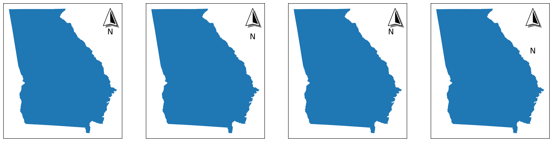
AOB
aob customizes the AnchoredOffsetBox object that handles the positioning of the final north arrow object with respect to the plot. Note that facecolor, edgecolor, and alpha are non-standard options.
| Attribute | Description | Accepts |
|---|---|---|
facecolor |
The color of the AnchoredOffsetBox patch. |
Any matplotlib color |
edgecolor |
The color of the edge of the AnchoredOffsetBox patch. |
Any matplotlib color |
alpha |
The transparency of the AnchoredOffsetBox patch. |
Any matplotlib color |
pad |
The amount of padding around the north arrow, defining the edges of the AnchoredOffsetBox. Expressed as a fraction of the fontsize specified in prop. |
Any positive number |
borderpad |
The amount of padding between the AnchoredOffsetBox and the bbox_to_anchor, if one is specified. Expressed as a fraction of the fontsize specified in prop. |
Any positive number |
prop |
A reference fontsize used to define the paddings of pad and borderpad. |
Any valid fontsize input |
frameon |
Whether or not to draw a frame around the box. | Either True or False |
bbox_to_anchor and bbox_transform |
Used to customize the placement of the AnchoredOffsetBox. |
See Tips and Tricks section for details |
# Modifying specific elements
modifications = [
    {"facecolor": "black"}, # different facecolor
    {"edgecolor": "red"}, # different edgecolor
    # these two show the difference between pad and borderpad
    {"edgecolor": "red", "pad": 3}, # increased pad
    {"edgecolor": "red", "borderpad": 3}, # increased borderpad
]

# Creating four subplots
fig, axs = new_map(1,4, figsize=(20,5))

for ax,m in zip(axs.flatten(), modifications):
    states.query(f"NAME=='Georgia'").plot(ax=ax)
    ax.set_aspect(1, adjustable="datalim")
    north_arrow(ax=ax, location="upper right", rotation={"degrees":0}, aob=m)
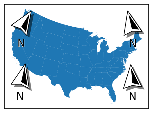
Rotation
rotation controls how the north arrow is rotated so that it points upwards (towards true north). There are two ways to customize this:
If the direction to north is not known, it can be automatically calcuated with three pieces of information:
| Attribute | Description | Accepts |
|---|---|---|
crs |
The coordinate reference system that the map is in. | Any pyproj CRS value (including strings and integers) |
reference |
The type of reference point from which north will be calcualted. | Any of axis, data, or center |
coords |
A tuple of coordinates from which north will be calculated. | Each coordinate can be either a float or an integer |
-
If
referenceisaxis, thencoordsshould be in axis coordinates, where(0,0)represents the bottom-left point of the plot, and(1,1)represents the top-right point of the plot. -
If
referenceisdata, thencoordsshould be in data coordinates, meaning that of the CRS supplied bycrs. -
If
referenceiscenter, then a value ofcoordsis not necessary - it is the equivalent of settingreferencetoaxisandcoordsto(0.5, 0.5). This is how most common software such as ArcGIS Pro and QGIS calculate the rotation of the north arrow.
# Demonstrating how the rotation changes based on the reference point
modifications = [
    ["lower left", {"crs":3520, "reference":"axis", "coords":(0.1, 0.1)}],
    ["upper left", {"crs":3520, "reference":"axis", "coords":(0.1, 0.9)}],
    ["upper right", {"crs":3520, "reference":"axis", "coords":(0.9, 0.9)}],
    ["lower right", {"crs":3520, "reference":"axis", "coords":(0.9, 0.1)}],
]

# Creating a single plot for the contiguous USA
to_exclude = ['Hawaii','Alaska','Guam','Commonwealth of the Northern Mariana Islands','United States Virgin Islands','American Samoa','Puerto Rico']

fig, ax = new_map(1,1, figsize=(4,6))

# Note that I'm using a CRS here that will create rotations explicitly! 3520 is really only suitable for Georgia.
states.query(f"NAME not in {to_exclude}").to_crs(3520).plot(ax=ax)

for m in modifications:
    north_arrow(ax=ax, location=m[0], rotation=m[1])
| Attribute | Description | Accepts |
|---|---|---|
degrees |
If a value is passed, the arrow will simply be rotated to that point; this can be used to point to other directions is necessary, or if the direction to north is known. | A number between -360 and 360 |
Tips and Tricks
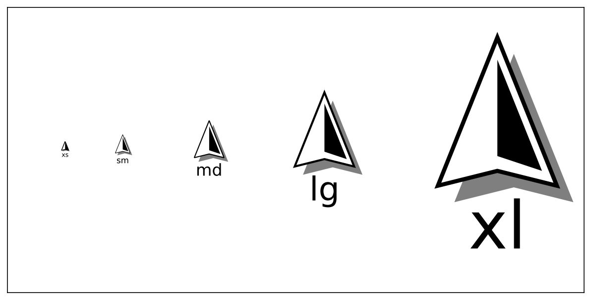
Setting Size
While the north arrow can nominally have its size changed by changing the scale attribute, doing so doesn't change the other, related components, such as the sizes of the text, the shadow's offset, the stroke widths, and so on.
However, given that there are standardized paper sizes that most graphics are made towards, a size parameter is available that will select pre-configured default values that approximate what looks best at each size. The parameter takes in only one input, which is the size tier you want:
-
xsmallorxsfor A8 paper, ~2 to 3 inches -
smallorsmfor A6 paper, ~4 to 6 inches -
mediumormdfor A4 or letter paper, ~8 to 11 inches -
largeorlgfor A2 paper, ~16 to 24 inches -
xlargeorxlfor A0 paper, ~33 to 48 inches
These default values can be seen in defaults/north_arrow.py.
# Creating an empty plot - for reference, this is 10 inches x 5 inches
fig, ax = new_map(1,1, figsize=(10,5))

# Visualizing the different sizes at various positions
for l,s in zip([0.1, 0.2, 0.35, 0.55, 0.85], ["xs","sm","md","lg","xl"]):
    # Using the size parameter to set the size directly
    north_arrow(ax=ax, size=s, location="center", label={"text":s}, rotation={"degrees":0}, aob={"bbox_to_anchor":(l, 0.5), "bbox_transform":ax.transAxes})
Placing Arrows Outside of Axis
Sometimes it is more desireable to place the arrow outside of the plot entirely, which can be accomplished using bbox_to_anchor and bbox_transform from the aobcomponent settings. This works the same way it does for matplotlib.pyplot.legend.
fig, ax = new_map()

states.query("NAME=='Georgia'").plot(ax=ax)

north_arrow(ax=ax, size="sm", location="upper left", rotation={"degrees":0}, aob={"bbox_to_anchor":(1.05,1), "bbox_transform":ax.transAxes})